Geometric Algebra

This post revisits the exterior product, forms and exterior derivative which was previously discussed in my vector spaces writeup. Revisting this section was necessary before coming to terms with the covariant exterior derivative when thinking about connections on fiber bundles which is discussed the next writeup.

In summary a vector is an element of a vector space and it is the properties of the space that are more important to us. With that in mind, a vector space is constructed where the following two properties hold:

The vectors are the elements for $a$ and $b$ for which the above is true but also notice there are the space of functionals ($f$) which also hold to the above properties given $a$ and $b$. This is the dual of the vector space and is also referred to as the covector space.

Also keep in mind is the ability to abstract multilinear maps which eat vectors (elements of a vector space) and covectors (elements of a covector space) to produce a scalar (element of the underlying field of the (co)vector space). These multilinear maps are called tensors. A tensor of particular interest to us is the n-form which is a multilinear map which eats n vectors and zero covectors to produce a scalar. We may also look at the set of all n-forms acting on a manifold $M$ which is denoted by $\omega_p \in \Omega^n(M)$.

Vectors in a vector space when equipped with a basis begin to take a very geometric intepretation. We can describe lines, parallelograms, volumes and planes in the language of vectors. Thus one can concieve it is useful to have a language which can algebraically manipulate these strcutures without having to really think about the geometry. This is the role of geometric algebra.

Exterior (wedge) product

I first introduced the exterior product as linear orientated area function which accepts any number of vectors with any dimension. The result is signed to maintain linearity.

Thinking purely in terms of the exterior product we can label new classes of mathematical objects called k-vectors (or blades). Elements of which include the 0-vector which is simply a scalar, vectors themselves, bivectors which are the orientated surface area spanned by two vectors, the trivector which is a combination of bivectors resulting in orientated volume and so on. By means of the exterior product to represent k-vectors we can algebraically work with concepts such as points, lines, areas and volumes.

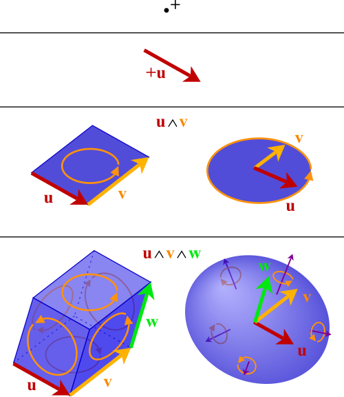
Furthermore by using combinations of k-vectors we can produce multivectors (i.e. linear combinations of scalars, vectors, bivectors and so on). It is k-vectors (wedge product vectors) which the building blocks to geometric algebra. Given we are working with combinations of k-vectors (multivectors) it is natural to define an operation to combine multivectors known as the geometric product.

Exterior product on forms

We know covectors and more generally forms are used to measure lines, areas and volumes. Therefore, similarly to how we construct higher order geometry by combinations of vectors and exterior products, so too can we construct the machinary to measure these higher order geomteries by means of the exterior product acting on forms.

To make forms more tangible consider its basis. Recall the basis for a tangent vector $X \in T_pM$ is $X = X^a \bigg(\frac{\partial}{\partial x^a}\bigg)_p$. For a differential form the basis is $\omega = \Set{dx^1, \dots, dx^n}$. Thus a form is a function of these basis which acts on n-vectors to produce a scalar.

Applications for the exterior product of forms inituitively becomes useful for integration which we are already familiar is useful for summing line segments, areas and volumes. However now in the language of geometric algebra we can describe an integral without making an assumption about the coordinate basis yet.

Exterior derivative of differential n-forms

To recap a n-form accepts n vectors and produces a scalar. Formally:

Now when we think about differential geometry, moving through a manifold we are interested the n-forms along every point. And even more specifically since it is differential geometry, the vectors for which these forms act on are the elements of the tangent space at each point. Thus a differential form is an assignment of a n-form to every point formally described below. Unfortunately, the formalism is a bit loose here from what I read/watched and the symbol $\omega$ is reused for both differetial forms and general forms.

With this in mind I can finally introduce an operation called the exterior derviative which acts on differential n-forms (assignment of forms along a manifold which act on elements within the tangent space at those respective points) and produces $(n+1)$-forms.

This was strange to me at first, since given some manifold why should I be able to algebraically construct a form with a higher grade (degree) from an existing form? It helps to remember that the exterior product is also a operation which allows us construct multivectors (higher grade vectors [e.g. bivectors become trivectors and so on]). We will see how introducing an operator to map a form to a higher grade ultimately generalizes already seen concepts such as gradient, curl and divergence which should already feel related because of their shared use of the $\nabla$ operator.

The definition for the exterior derivative is given as follows:

Most of the space taken is because we have to generalize the number of parameters. The formula simply tells us how to construct a new form $d\omega$ that accepts $n+1$ tangent vectors written in terms of orignal form $\omega$. The first alternating sum simply picks a tangent vector $X_i$ and applies the operation (differentiate) the orginal form $\omega$ acting on the other tangent vectors (remember number of paramters accepted by $\omega$ is still the same since omitting $X_i$) in the direction of $X_i$. If we take $\omega$ to be a 1-form we get $X_1\omega(X_2) - X_2\omega(X_1)$. This operation alone is not linear when applied to $C^\infty(M)$ functions. If $X_i$ and $X_j = gX_i$ are in the same direction then the first summation part is not necessarily zero even though it should be, as shown below:

The second alternating sum is a correction factor to address this. It being a correction factor is hinted at given the appearance of the Lie bracket (commutator) of the tangent operators (vector fields) $X_i$ and $X_j$ which produces a new vector field that measures by how much the commutative property of the operators $X_i$ and $X_j$ fails. Thus we have a new form $d\omega$ with one extra parameter (higher grade) written in terms of the orginal differential form $\omega$.

Now to relate to gradient fields, curl and divergence look at the following three examples, which select a form (starting at grade 0 and progressively get higher) and see what the resulting form is after applying the exterior derivative.

The first case is to introduce a 0-differential form (just a function $f$) for $\omega$ as follows acting on a vector field $\vec{F} = P\hat{i} + Q\hat{j} + R\hat{k}$ and see that the exterior derivative $d\omega$ produces a 1-form which we can recognize as the gradient field.

Now let $\omega$ be a differential 1-form and we can see the exterior derivative $d\omega$ produces a 2-form analogous to the curl of a vector field.

Now let $\omega$ be some two form (whose basis are the bivectors below) and we will see how it becomes a three form similar to the definition of divergence.

deRham cohomology

Starting with any n-form (any grade), we can prove that applying the exterior derivative operator twice to that n-form will produce $0$. It leads to real-world intepretations such as the curl of a gradient field is zero and the divergence of curl is zero.

Generalized Stoke’s theorem

Putting it all together, a generalized version of Stoke’s theorem can be written. To recap, Green’s theorem relates the line integral of a curve $C$ to the flux passing through the area $A$ of the region enclosed by the curve $D$ for a vector field $\vec{F} = P\hat{i} + Q\hat{j}$ in $\R^2$ as follows:

Stoke’s theorem generalizes Green’s theorem in a higher dimension $\R^3$ where the line $C$ is described using vectors $\vec{r}$ and instead of the “area” in $R^2$ we look think about the flux passing through a surface $S$.

A limitation of the above two theorems is that we may want to generalize to dimensions higher than $R^3$. Furthermore the area/surface under question must have no holes in them. I have discussed in aprevious post how a topology can be classified by the number of holes it has (i.e. the homology group). The generlaized Stoke’s theorem below written in terms of differential forms removes these limitations.